 《HEARIM · 헤아림》 Vol.1 No.1·Research Article·Published 2026-09-28·First posted: ScholarBridge Lab working paper·PDF (EN)
AI use: Korean edition machine-translated (Claude/Codex) and checked number-for-number against this English original; authoring disclosure pending
Why this is our first paper → Cover
Tail Thickness, Not Accuracy: A Label-Free Screen for Delegating Judgments to Cheap Probability Models

Judgment-only models that return a probability for a fixed proposition are now cheap enough to sit in front of every expensive decision. The natural deployment is a two-threshold gate: act automatically when the probability is near 0 or 1 and escalate the middle to a stronger model or a person. We argue that the quantity that decides whether such a gate pays is not accuracy but tail thickness \(\tau\), the fraction of inputs whose returned probability falls at or below 0.10 or at or above 0.90. Because \(\tau\) depends only on the score distribution, it can be measured on unlabeled inputs and bounds, before any labeling, the share of escalation cost the gate can remove. Prior pilot measurements on one cheap judgment model motivate the screen: on 120 real e-mails the model was honest at the extremes but non-monotone in the middle and placed only 5% of inputs in the tails; on 24 essay paragraphs \(\tau\) fell from 83% for a mechanical factual question to 0% for two preference questions, and writing an explicit rubric into a preference question left \(\tau\) at 0%. We then report five pre-registered experiments. A counting control yields \(\tau\) = 8.3% (4.2% in a balanced re-test), so the rubric result is confounded. Across seven questions ordered from factual to preferential on 96 paragraphs, Spearman \(\rho\) between declared order and \(\tau\) is −0.955; both preference questions have \(\tau\) = 0% with upper 95% bounds of 0. Test–retest median \(|\Delta p|\) is 0.01 at worst. A general LLM shows \(\tau\) = 85% on the importance question and 17.7% error inside its tails on the factual one, and the mail-data monotonicity permutation test gives \(p\) = 0.045, contradicted by an exploratory statistic. Thin tails are therefore best read as calibrated caution: \(\tau\) is a cheap, label-free first screen that bounds a gate’s saving, but it must be paired with a check of the error inside the tails.
1 Introduction
A new class of model sells judgment rather than text. Given an input and a pre-specified proposition (“this e-mail is unwanted bulk advertising”, “this paragraph contains a number”), it returns a single probability. The model studied here, Jev 1.13 (TypeSafe AI, released September 2026), is priced at USD 0.042 per million input tokens with free output; in our first pilot the median latency was 418 ms and the full 120-item benchmark cost less than USD 0.002 (Insight Lab 2026b). At this price the cost of asking is negligible, and the vendor’s claim is that the returned probability is calibrated: an answer of 0.9 should be right nine times in ten.
If that claim held uniformly, the economics would be simple. Cheap judgments would be used everywhere, in the spirit of Jevons’ observation that efficiency gains raise total consumption (Jevons 1865). The engineering pattern that makes this concrete is the cascade: a cheap stage decides the easy cases and passes the rest to an expensive stage (Viola and Jones 2001; Chen et al. 2023). For a probability-returning model the cascade reduces to a two-threshold gate, auto-accept above \(1-t\), auto-reject below \(t\), escalate in between, which is the classical reject option (Chow 1970) and the selective-classification setting (Geifman and El-Yaniv 2017).
Whether a gate is worth building is usually decided by accuracy or by a calibration curve. Both require labels, and both average over the region the gate never uses. Our pilot data show why this is the wrong order of questions. On 120 real e-mails the model was 62% accurate, its extreme bins were honest (8% spam below 0.2, 100% above 0.8), and its middle bins were inverted (58% spam in 0.2–0.4 versus 17% in 0.4–0.6) (Insight Lab 2026b). More decisive than either fact was that only 6 of 120 answers (5%) reached the \(\le 0.10\) or \(\ge 0.90\) region. A gate at those thresholds made no errors and escalated 95% of the traffic (Insight Lab 2026a).
This paper proposes to screen tasks by that last number first. Our contributions are:
- A label-free screen. We define tail thickness \(\tau\) and show that it upper-bounds the fraction of escalation cost a two-threshold gate can save, using only unlabeled inputs (Section 3).
- A task-level hypothesis with a paradox. Pilot measurements suggest that \(\tau\) tracks how factual the question is, falling to 0% for preference questions. The tasks with thick tails are the ones that rules already solve; the tasks that resist rules have no tails (Insight Lab 2026a).
- A negative pilot result. Writing an explicit rubric into a preference question widened the score spread but did not create tails (0% before and after).
- Five pre-registered experiments (E1–E5, plus a registered addendum E1b) that test the screen’s assumptions: whether the model can be confident on a computable fact at all, whether \(\tau\) decreases with preferentiality at \(n = 96\), whether single calls are stable enough for fixed thresholds, whether thin tails are specific to this model, and whether the mail-data non-monotonicity survives a permutation test. All outcomes, including failures, are reported against rules fixed before data collection.
3 Method
3.1 Tail thickness
Let a judgment model return \(p(x) \in [0,1]\) for a fixed proposition and input \(x\). For thresholds \(t_\ell < t_h\), define
\[ \tau(t_\ell, t_h) \;=\; \Pr_x\!\left[\, p(x) \le t_\ell \;\lor\; p(x) \ge t_h \,\right], \]
estimated by the sample fraction. Throughout, \(t_\ell = 0.10\) and \(t_h = 0.90\), and we write \(\tau\). We report the lower and upper tails separately when they differ in operational meaning (for instance, when only auto-accept is safe).
Why it is label-free. \(\tau\) is a functional of the marginal distribution of \(p(x)\) alone. It can be computed on any unlabeled sample of the deployment input stream. Labels are needed only to estimate the error inside the tails, and that sample has size \(\tau n\), so a thin-tailed task costs almost nothing to reject and a thick-tailed task needs labels only for the items the gate would act on.
3.2 Gate economics
Consider a two-threshold gate. Every item incurs the cheap call cost \(c_J\); the fraction \(1-\tau\) is escalated at cost \(c_E\); tail items decided automatically are wrong with rate \(\varepsilon\) at loss \(L\) each. Relative to escalating everything, the expected saving per item is
\[ S \;=\; \tau\,(c_E - \varepsilon L) \;-\; c_J , \qquad \frac{S}{c_E} \;\le\; \tau . \]
Two consequences follow. First, whatever the tail error, the saved fraction of escalation cost is at most \(\tau\); this bound is available before labeling. Second, the per-call price enters only through \(c_J/c_E\). With the price ratio used in the pilot (about 225-fold, 0.002 versus 0.45 US cents per judgment, where the LLM figure is a published comparison on a different task, customer-inquiry classification, and serves only as an order-of-magnitude guide (Insight Lab 2026b)), \(c_J/c_E \approx 0.004\), so the API cost of the cheap model is not the binding constraint; the binding constraints are \(\tau\), the error \(\varepsilon\) in the tails, and fixed costs outside this expression (integration, added latency on the \(1-\tau\) escalated items, monitoring). A task with \(\tau = 5\%\) can at best remove 5% of escalation cost, which rarely justifies a second system in the loop.
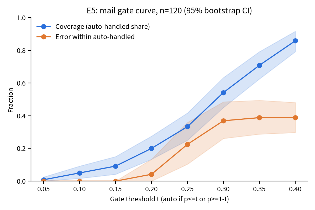
Loosening the thresholds is not free. When \(\tau\) is small, the temptation is to widen the tails. In the mail pilot, auto-deciding \(p \le t\) or \(p \ge 1-t\) gave coverage/error of 9%/0% at \(t=0.15\), 20%/4.2% at \(t=0.20\) and 33%/22.5% at \(t=0.25\) (Insight Lab 2026a). Error grows abruptly rather than smoothly because of the next requirement.
3.3 Monotonicity requirement
A threshold rule presumes that \(\Pr[y=1 \mid p]\) is non-decreasing in \(p\). If it is not, moving a threshold inward admits a region in which the score does not even order items correctly, and no choice of \(t\) inside that region is principled. In the mail pilot the empirical bin rates were 8%, 58%, 17%, 62% and 100% for \(p\) in \([0,0.2)\), \([0.2,0.4)\), \([0.4,0.6)\), \([0.6,0.8)\) and \([0.8,1]\), with bin sizes 12, 52, 23, 21 and 12 (Insight Lab 2026b): honest at the ends and inverted in the middle. Isotonic recalibration (Zadrozny and Elkan 2002) can force monotonicity but only by pooling the violating bins, which removes resolution rather than adding it. We therefore treat thick tails as necessary, and monotonicity near the thresholds plus low tail error as the additional conditions, checked with labels only on the \(\tau n\) tail items. Experiment E5 asks whether the observed violations exceed what shuffled scores would produce.
3.4 Pre-registration
The protocol for E1–E5 was fixed on 2026-09-27, before any E1–E5 data existed, in a file whose SHA-256 digest (74bbd759…d7d9145a) was recorded at registration. It fixes the model, corpus, question sets, the tail definition, all decision thresholds and the budget ceiling. Each hypothesis is reported as supported, not supported or inconclusive exactly by the registered rules; no wording, threshold or sample is changed after seeing data, and any deviation is listed in a dedicated section. The two earlier pilot probes followed the same practice informally: their decision thresholds (e.g. \(\tau \ge 15\%\) to support the rubric hypothesis) were written into the probe scripts before the runs.
4 Experimental Setup
4.1 Model and interface
All Jev experiments use Jev 1.13 (TypeSafe AI) accessed through OpenRouter via the vendor’s System One API, which takes an input state and a set of named propositions and returns one probability per proposition in a single call. Prompts are zero-shot. No other property of the model is assumed. A spending ceiling of USD 1.50 across all runs was registered as a stopping rule.
4.2 Data
Mail (E5 only). The 120 real e-mails of the first pilot (60 legitimate, 60 spam; labels from the mail service’s own folder assignment; the model saw sender domain, subject and the first 500 characters of the body) (Insight Lab 2026b). Only labels and returned probabilities are retained; E5 makes no new calls.
Paragraphs (E1–E4). Paragraphs of the public Insight Lab journal (Korean science essays), 200–700 characters, excluding tables and mathematics, extracted with the same rule as the earlier tail probe. The corpus as run also contained unpublished drafts by the same author (see Deviations). Raw outputs store only paragraph index and length, never text.
4.3 Prior pilot measurements
For context and to make the registered hypotheses traceable, we summarize the already published probes. In the tail probe (Insight Lab 2026a) (\(n=24\) paragraphs, five propositions in one call), \(\tau\) was 83% for has_number (“This text contains at least one numeral or numeric figure”; tail error 0, overall agreement 96% against a regular-expression ground truth), 33% for is_method, 29% for has_counter, and 0% for both preference propositions is_important (range 0.48–0.78) and should_shorten (range 0.22–0.36). In the rubric probe (same corpus rule, \(n=24\)), each preference proposition was asked twice, as originally worded and with an explicit author’s rule (importance: states a measured result, the main claim or a counter-interpretation; shortening: longer than 400 characters and redundant or carrying unneeded background). Under the registered criterion (\(\tau \ge 15\%\) supports the rubric hypothesis) the hypothesis was rejected: \(\tau\) stayed at 0% for both, although the score range of is_important widened from 0.29 to 0.62 (and of should_shorten from 0.16 to 0.23). This result is ambiguous: the shortening rubric contains a computable length condition, so the failure could reflect preference framing or an inability to judge length at all. E1 was registered to resolve this.
4.4 Experiments
E1 — counting versus framing. The same 24 paragraphs as the rubric probe, proposition “This text is longer than 400 characters” (truth computable). If \(\tau \ge 40\%\) and tail-region error is 0, the model can judge length and the rubric result is attributed to preference framing. If \(\tau < 15\%\), the model cannot judge length reliably and the rubric result is reported as confounded. Values in between are inconclusive. (In the rubric-probe sample only one of the 24 paragraphs exceeds 400 characters, so this control mostly tests confident negatives.)
E2 — scale-up with uncertainty (main result). \(n = 96\) evenly sampled paragraphs, seven propositions in one call per paragraph, in a declared order from most factual to most preferential: (1) has_number, (2) has_latin_word, (3) is_method, (4) has_counter, (5) states_main_claim, (6) is_important, (7) should_shorten. For each proposition we report \(\tau\) with a bootstrap 95% CI (2,000 resamples) (Efron 1979). Hypotheses: H2a, Spearman \(\rho\) between declared order and \(\tau\) is negative; H2b, the upper CI bound of \(\tau\) is at most 0.10 for both preference propositions (6, 7); H2c, for the two propositions with free ground truth (1, 2) the tail-region error rate is at most 5%.
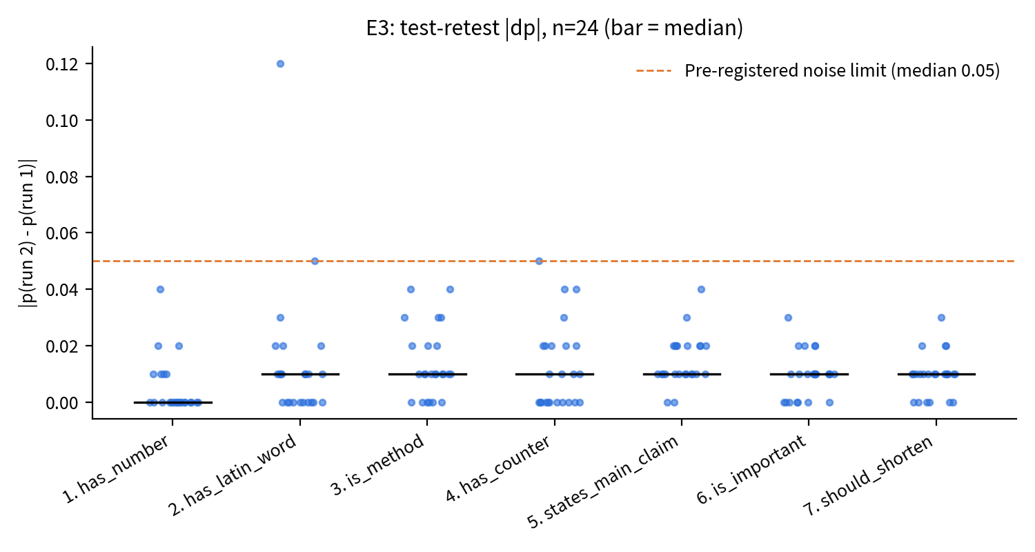
E3 — test–retest stability. The first 24 paragraphs of E2 are submitted again in a second, separate run with identical inputs. We report the median and 90th percentile of \(|\Delta p|\) per proposition. If the median exceeds 0.05 for any proposition, a single call is declared too noisy for fixed-threshold gating of that proposition.
E4 — cross-model specificity. The same 96 paragraphs, propositions 1, 4 and 6, are asked to a general LLM (gpt-5.6-luna, via a local command-line tool) with a prompt requesting a single probability in \([0,1]\) as JSON. We report \(\tau\) and, for proposition 1, tail-region error. If the general LLM shows \(\tau \ge 15\%\) on proposition 6 while Jev shows approximately 0%, and the LLM’s tail-region error on proposition 1 exceeds 5%, we interpret the LLM as overconfident rather than Jev as under-confident. Any other pattern is reported descriptively without further claim.
E5 — mail re-analysis (no new calls). Bootstrap 95% CIs of \(\tau\) and of the gate error curve for thresholds \(t \in [0.05, 0.40]\). Monotonicity is assessed by comparing observed bin rates with an isotonic fit (Zadrozny and Elkan 2002) and by a permutation test (5,000 shuffles of the scores) of the number of monotonicity violations, at \(\alpha = 0.05\).
E1b — balanced length test (registered addendum). Because the E1 sample has only one positive item, a 24-paragraph sample with 12 paragraphs above and 12 at or below 400 characters was registered as an addendum before the registrant saw any E1 result, with the same proposition and decision rule. Accuracy at \(p \ge 0.5\) is reported separately for the two groups.
Reporting. Total spend was about USD 0.029 (Jev USD 0.0035 for 144 calls; gpt-5.6-luna an estimated USD 0.025 for 288 calls), well below the ceiling. Deviations from the protocol are listed in the Results section.
5 Results
All numbers below are taken from the saved run outputs; percentages are shares of items, and CIs are bootstrap percentile intervals (2,000 resamples, seed 20260927). Table 1 collects every registered hypothesis and its verdict.
| Exp. | Registered hypothesis / rule | Key result | Verdict |
|---|---|---|---|
| E1 | \(\tau \ge 40\%\) with 0 tail error → framing; \(\tau < 15\%\) → confounded | \(\tau\) = 8.3% [0.0, 20.8] | confounded |
| E1b | same rule, balanced 12 + 12 sample | \(\tau\) = 4.2% [0.0, 12.5] | confounded |
| E2 H2a | Spearman \(\rho\)(order, \(\tau\)) < 0 | \(\rho\) = −0.955 | supported |
| E2 H2b | upper 95% bound of \(\tau\) ≤ 0.10 for q6, q7 | 0.0 and 0.0 | supported |
| E2 H2c | tail-region error ≤ 5% for q1, q2 | 3.6% (3/84) and 0% (0/57) | supported |
| E3 | median \(|\Delta p|\) > 0.05 → too noisy | max median 0.01 | no proposition too noisy |
| E4 | LLM \(\tau_6 \ge 15\%\), Jev \(\tau_6 \approx 0\), LLM q1 tail error > 5% → LLM overconfident | 85.4%, 0%, 17.7% | rule met: LLM overconfident |
| E5 | permutation test of monotonicity violations, \(\alpha = 0.05\) | 2 violations, \(p\) = 0.045 | significant (borderline) |
5.1 E1 — counting versus framing
In the 24 rubric-probe paragraphs, only 1 exceeds 400 characters. Jev placed 2 of 24 answers in the tails (\(\tau\) = 8.3%, 95% CI [0.0, 20.8]); both were correct (tail-region error 0/2). Scores ranged from 0.09 to 0.82 (median 0.32); the mean score was 0.50 for the one long paragraph and 0.34 for the others. Accuracy at a 0.5 cut was 83.3%, below the 95.8% of always answering “no”. Since \(\tau < 15\%\), the registered verdict is confounded: the model cannot judge the length proposition reliably, and the rubric-probe null result cannot be attributed to preference framing. The positive class has \(n = 1\), which motivated E1b.
5.2 E1b — balanced length test (registered addendum)
The corpus contains 21 paragraphs longer than 400 characters and 276 of 400 or fewer; the sample took 12 of each. \(\tau\) was 4.2% (95% CI [0.0, 12.5]) with tail-region error 0/1, and all scores lay between 0.10 and 0.64. Accuracy at \(p \ge 0.5\) was 42% in the long group and 92% in the short group: the model defaults to “not longer”. The registered verdict is again confounded. Together, E1 and E1b show that Jev does not count characters, so the rubric-probe result cannot be used to separate preference framing from an inability to evaluate the length condition.
5.3 E2 — tail thickness across seven propositions
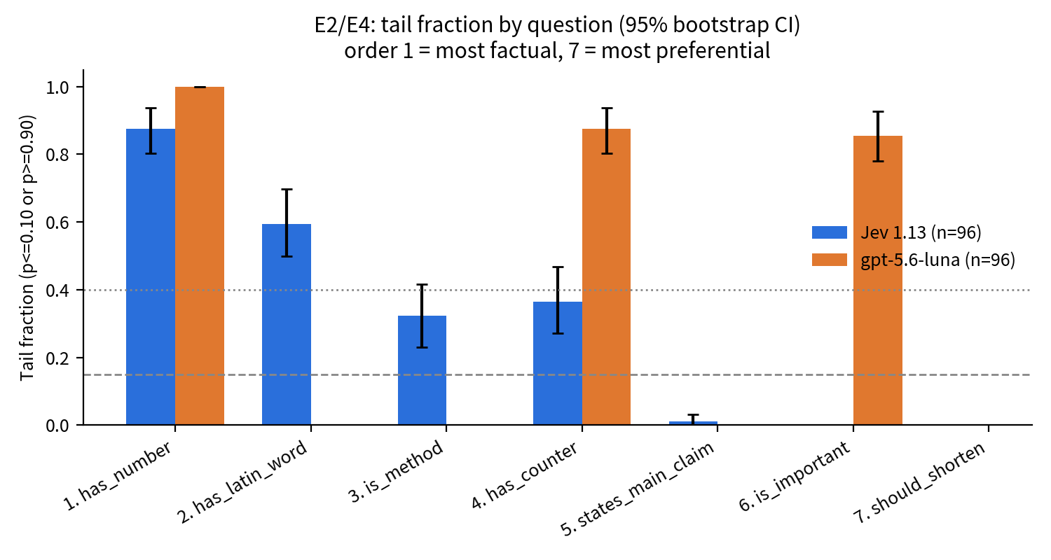
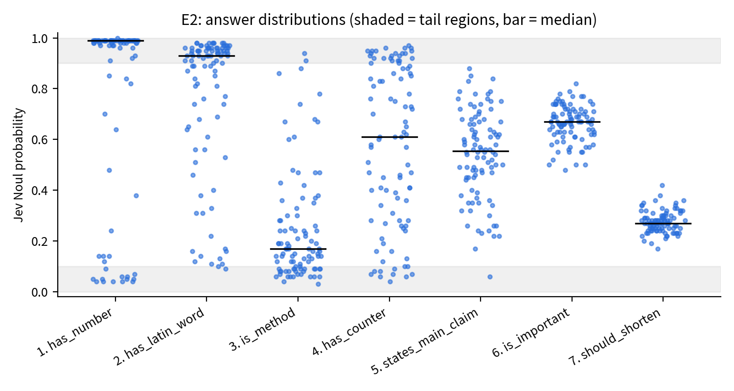
All 96 calls succeeded. Table 2 and Figure 1 give \(\tau\) per proposition; Figure 2 shows the score distributions.
| # | Proposition | \(\tau\) | 95% CI | \(p \le .10\) | \(p \ge .90\) | min / median / max | tail-region error |
|---|---|---|---|---|---|---|---|
| 1 | has_number | 87.5% | [80.2, 93.8] | 13.5% | 74.0% | 0.04 / 0.99 / 1.00 | 3/84 = 3.6% [0, 8.1] |
| 2 | has_latin_word | 59.4% | [50.0, 69.8] | 2.1% | 57.3% | 0.09 / 0.93 / 0.98 | 0/57 = 0% |
| 3 | is_method | 32.3% | [22.9, 41.7] | 30.2% | 2.1% | 0.03 / 0.17 / 0.94 | – |
| 4 | has_counter | 36.5% | [27.1, 46.9] | 11.5% | 25.0% | 0.04 / 0.61 / 0.97 | – |
| 5 | states_main_claim | 1.0% | [0.0, 3.1] | 1.0% | 0% | 0.06 / 0.56 / 0.88 | – |
| 6 | is_important | 0.0% | [0.0, 0.0] | 0% | 0% | 0.48 / 0.67 / 0.82 | – |
| 7 | should_shorten | 0.0% | [0.0, 0.0] | 0% | 0% | 0.17 / 0.27 / 0.42 | – |
H2a is supported: Spearman \(\rho\) between declared order and \(\tau\) is −0.955. H2b is supported: the upper 95% bounds for is_important and should_shorten are both 0.0; no answer to either came within 0.07 of a tail threshold. H2c is supported on the registered point estimates (3.6% for has_number, 0% for has_latin_word; accuracy at 0.5 was 94.8% and 91.7%). The evidence for has_number is not tight: its bootstrap upper bound (8.1%) exceeds 5%. The three errors were one paragraph containing digits scored 0.05 and two paragraphs without digits scored 0.97. Restricted to the 41 paragraphs from published essays (see Deviations), \(\tau\) for propositions 1–7 was 87.8, 51.2, 31.7, 41.5, 0.0, 0.0 and 0.0% with \(\rho\) = −0.927, leaving H2a and H2b unchanged.
5.4 E3 — test–retest stability
Re-submitting the first 24 E2 paragraphs in a separate run changed scores very little (Figure 3). The median \(|\Delta p|\) was 0.00 for has_number and 0.01 for each of the other six propositions; the 90th percentiles were 0.02–0.04 and the largest single change was 0.12 (has_latin_word). No answer crossed a tail threshold between runs. No proposition exceeds the registered 0.05 median, so a single call is not declared too noisy for fixed-threshold gating of any proposition.
5.5 E4 — cross-model comparison
gpt-5.6-luna answered all 288 prompts in parseable form. Its \(\tau\) was 100% [100, 100] on has_number, 87.5% [80.2, 93.8] on has_counter and 85.4% [78.1, 92.7] on is_important, against Jev’s 87.5%, 36.5% and 0.0% (Figure 1). On has_number its tail-region error was 17/96 = 17.7% (Jev 3.6%), accuracy at 0.5 82.3%. All three registered conditions hold, so the registered interpretation applies: the general LLM is read as overconfident, not Jev as under-confident. Sixteen of luna’s 17 errors assert a numeral at \(p \ge 0.98\) for paragraphs without an ASCII digit; some of these contain Korean number words (e.g. 세 가지, “three kinds”). Under an exploratory, broader truth (“ASCII digit or Korean number word”) the tail-region errors become 11.5% (11/96) for luna and 7.1% (6/84) for Jev. The registered interpretation still holds (11.5% > 5%), but the gap between the models shrinks from about fivefold to about 1.6-fold. On the 8 paragraphs with number words and no digit, Jev’s scores were spread from 0.04 to 0.97, so Jev was not consistently committed there either.
5.6 E5 — mail re-analysis
On the 120 mails (60 junk), \(\tau\) = 5.0% (95% CI [1.7, 9.2]); scores ranged from 0.08 to 0.98 (median 0.36). Figure 4 shows the gate curve. Error among auto-decided mails was 0% up to \(t = 0.15\) (coverage 9.2% [4.2, 15.0], 11 mails), 4.2% [0, 13.3] at \(t = 0.20\) (coverage 20.0%), 22.5% [10.3, 35.9] at \(t = 0.25\) (coverage 33.3%), and 36.9–38.8% for \(t = 0.30\)–\(0.40\) (coverage 54–86%).
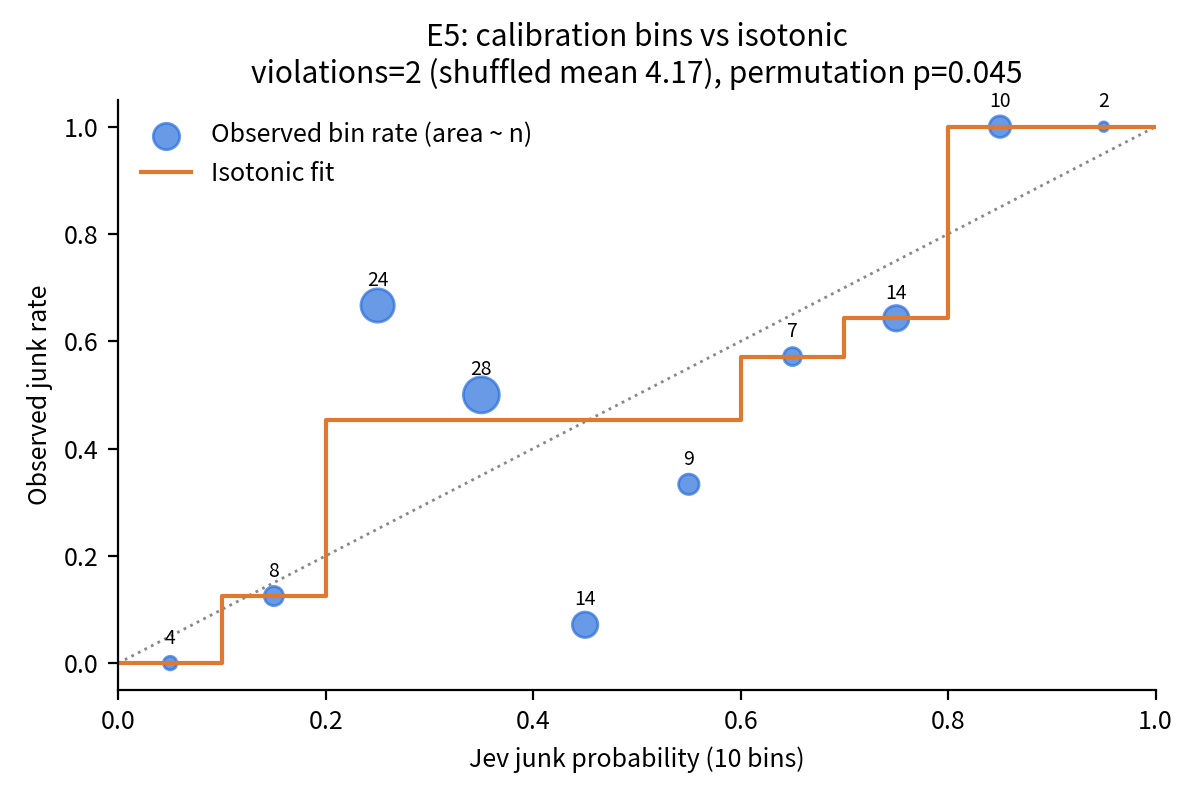
In ten equal-width bins the junk rates were 0.00, 0.13, 0.67, 0.50, 0.07, 0.33, 0.57, 0.64, 1.00 and 1.00 (bin sizes 4, 8, 24, 28, 14, 9, 7, 14, 10, 2; Figure 5). There were 2 adjacent decreases against a shuffled-score mean of 4.17; the one-sided permutation \(p\) (5,000 shuffles) is 0.045, significant at \(\alpha = 0.05\): the score ordering has fewer monotonicity violations than shuffled scores. This is borderline, and it does not mean the curve is monotone: the 0.2–0.5 region (66 mails, 55%) is inverted (0.67 → 0.50 → 0.07), and the isotonic fit pools the bins from 0.2 to 0.6 at 0.45. An exploratory statistic that measures the size of the departure rather than the count (see Deviations) points the other way (\(p\) = 0.94). The reference labels are a further caveat: of the 19 folder-labelled legitimate mails in the 0.4–0.6 band, 12 are ones the model itself classed as newsletters or marketing, that is, bulk mail the provider delivered to the inbox. Part of the apparent inversion may therefore be noise in the reference (folder placement) rather than a property of the scores.
5.7 Deviations from the pre-registration
- E5 analysis details were fixed by the executor before running E5, because the protocol did not specify them: a symmetric gate \(p \le t\) / \(p \ge 1-t\) with \(t = 0.05, 0.10, \dots, 0.40\); ten equal-width bins; a violation defined as an adjacent decrease in bin rate; and a one-sided \(p = \Pr(V_\text{perm} \le V_\text{obs})\) with scores shuffled across mails.
- Unregistered E5 statistic. In addition, the executor computed the weighted squared distance of the bin rates to the isotonic fit (3.32), with permutation \(p = \Pr(\text{perm} \le \text{obs}) = 0.94\), i.e. the departure from monotonicity is larger than under most shuffles. This statistic is exploratory. The two statistics disagree: the registered violation count says the ordering is better than chance, while the size of the departure is not. Any conclusion about monotonicity therefore depends on the statistic chosen.
- E4 transport. gpt-5.6-luna was called through the OpenAI API directly rather than through OpenRouter, with reasoning effort “low” (the tool’s default), a 1,000-token output limit and a one-line system message requesting JSON only. Its cost is the tool’s token-price estimate.
- E1b first run invalid. A script bug sent a (file, text) tuple instead of the paragraph text, so the measured length was 2. That run was discarded and E1b was re-run with the identical registered protocol; the discarded output is retained separately and marked invalid.
- E1b registration timing. E1b was registered at 18:45, after PREREG (18:39). At that time the E1 output file already existed on disk, but the registrant had not opened it.
- Corpus. The protocol described the corpus as the public Insight Lab journal. The file glob on the executing machine also matched five unpublished draft essays by the same author: 170 of the 297 corpus paragraphs and 55 of the 96 E2 paragraphs came from these drafts, and they were sent to the Jev and OpenAI APIs. They contain no third-party or employer data. The public-only subset (\(n = 41\)) gives \(\rho\) = −0.927 and \(\tau_6 = \tau_7 = 0\) (E2 subsection), so H2a and H2b are unchanged.
- Minor. E3’s “separate run” was a separate process started a few minutes after E2 with identical inputs. Bootstrap CIs for the E1 tail and the E2/E4 tail-region errors, accuracy at 0.5, the public-only subset and the broad-truth E4 re-scoring are additions, not registered tests. The Jev runner allowed one retry per paragraph on exception; none occurred.
No proposition wording, threshold or sample was changed after seeing data.
6 Discussion
(a) Tail thickness tracks factuality. Across seven propositions, \(\tau\) fell almost monotonically with declared preferentiality (\(\rho\) = −0.955): 88% for has_number, 59% for has_latin_word, 32–37% for the two semantic propositions, and 0–1% for the three that require the reader’s judgment. The ordering was fixed before data collection, it held on the public-only subset, and single calls were stable enough (E3) that the pattern is not sampling noise of the model. The intermediate band (propositions 3 and 4) separates from both ends by its CIs.
(b) The paradox. The propositions with thick tails are the ones a rule already solves: has_number is a regular expression, and it is also the only proposition on which we could compute a free ground truth. The propositions that resist rules (is_important, should_shorten, states_main_claim) had essentially no tails. In this setting, the cheap judgment model is confident exactly where it is least needed, and a gate at 0.10/0.90 would act on almost none of the items where a rule is unavailable.
(c) The general LLM fails the opposite way. gpt-5.6-luna committed almost always: 100% of its has_number answers and 85% of its is_important answers were in the tails, including 17 confident errors on the factual proposition. A tail-based gate on luna would have high coverage and would pass those errors through. Against this, Jev’s thin tails on preference propositions read as calibrated caution rather than as under-confidence, which is the registered E4 interpretation. Two qualifications apply: the broader truth definition narrows the factual-error gap to about 1.6-fold, and the two models received different prompt formats. The practical lesson is that \(\tau\) alone cannot distinguish useful confidence from overconfidence; a tail-based gate must be paired with a check of the error inside the tail region.
(d) What the rubric result can and cannot say. The pilot rubric widened the score spread of is_important but did not create tails. We registered E1 to decide whether this was because preference framing suppresses confidence or because the shortening rubric contained a length condition the model could not evaluate. Both E1 and the balanced E1b were confounded: Jev cannot count characters and defaults to “not longer”. We therefore could not separate framing from counting, and the rubric-probe null remains uninterpretable on that point.
(e) A practical recipe. Measure \(\tau\) without labels on roughly 24–96 items of the real input stream; the E2 CIs at \(n = 96\) were at most about ±10 points, and E3 suggests one call per item suffices. If \(\tau\) is small, stop: the escalation cost the gate can save is bounded above by \(\tau\) (Section 3). If \(\tau\) is large, spot-check the tail-region error with a few labels drawn only from tail items, and check that the score ordering near the thresholds is monotone. This corrects a claim in our earlier pilot: SP26 (Insight Lab 2026a) described a gate with 5–10% tails as a “pure loss”. That overstated the case. Because the cheap call is about two orders of magnitude cheaper than the escalation it screens, its added API cost is negligible; the correct statement is that the saving is bounded above by \(\tau\), which is small but not negative, and that fixed integration and monitoring costs, not the per-call price, decide whether it is worth building.
7 Limitations
- One cheap model. All Jev results come from one version of one judgment model, zero-shot; the comparison is one general LLM.
- One language and corpus. Korean science essays and one mail sample; a single author wrote the essays, the prior pilots and this paper.
- Unpublished drafts in the corpus. More than half of the E2 paragraphs came from the author’s unpublished drafts. The public-only subset gives the same qualitative result but is small (\(n = 41\)).
- Small \(n\). 24–120 items; E5 bins contain 2–28 mails, and the H2c upper bound for has_number (8.1%) exceeds the 5% criterion.
- Truth definition for has_number. The registered truth is an ASCII digit. Korean number words change both models’ error rates (E4 subsection), and the Jev–luna gap depends on this choice.
- Different prompt formats. luna received a free-text prompt asking for a JSON probability, whereas Jev received named propositions through its structured API; part of the tail difference may be format.
- Borderline E5. The registered monotonicity test gives \(p\) = 0.045, and an exploratory statistic gives \(p\) = 0.94; we do not regard monotonicity of the mail scores as established.
- Unbalanced E1. The registered E1 sample had one positive item; E1b, registered as an addendum, addresses this but is also small (\(n = 24\)).
- Fixed thresholds. Only 0.10/0.90 was registered; mail labels come from the mail service’s folders.
8 Conclusion
Tail thickness can be measured without labels and bounds what a two-threshold gate can save. In five pre-registered experiments and one registered addendum, it decreased with the preferentiality of the proposition (\(\rho\) = −0.955), was 0% for preference propositions, and was stable across repeated calls. A general LLM showed the opposite pattern, committing to extreme probabilities including where it was wrong. We could not separate preference framing from the model’s inability to count, and the mail-data monotonicity result depends on the statistic chosen. The screen we recommend is modest: measure \(\tau\) first, then check error inside the tails before building the gate.
Data and Code Availability
The experiment scripts, the pre-registration files with their SHA-256 digests, and the anonymised JSON outputs (paragraph index, length, ground-truth flags and returned probabilities; mail labels and probabilities) are kept in the author’s archive and are available from the author on request. No paragraph text or e-mail content is stored in the released data.