 《HEARIM · 헤아림》 Vol.1 No.1·Research Article·Published 2026-09-28·PDF (EN)
AI use: Korean edition machine-translated (Claude/Codex) and checked number-for-number against this English original; authoring disclosure pending
What a Circuit Cannot Do: Locating the Term that Carries Multifractality in Capital Flow, and the Portfolio Consequences of Finding It

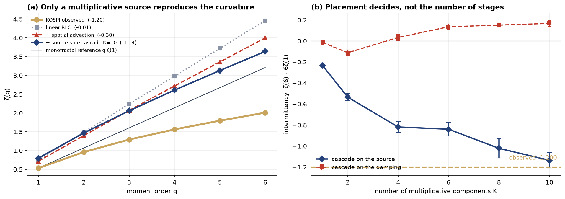
A capital-flow model written in the form of the Navier–Stokes equations is tested term by term against KOSPI data and then against twenty-six years across five markets. The analogy fails where it is usually invoked and holds where it is not. The model’s own Reynolds number falls through a crash, so its own formula classifies a \(38.6\%\) decline as laminar; viscosity and cross-sectional gradient peak 28 and 34 trading days after the price peak, so neither leads. What does hold is scaling: structure-function exponents are distinctly concave, with intermittency \(\zeta(6)-6\zeta(1)=-1.397\) and a block-bootstrap 95% interval of \([-1.991,-0.551]\). We then locate the responsible term. A passive linear network cannot produce that curvature, because superposition makes stage currents add rather than multiply; neither a current-dependent resistor nor a ladder of geometrically spaced stages succeeds. Spatial advection on a transmission line produces intermittency for the first time (\(-0.303\pm0.026\)) but reaches a quarter of the observed value. A multiplicative cascade acting on the driving source rather than on the damping reproduces it, \(-1.136\pm0.074\) at ten components, and lowers out-of-sample reconstruction error by \(48.9\%\) across 103 held-out windows in five markets (Wilcoxon \(p=0.0027\)). The improvement does not reach the portfolio. The same multi-scale structure forecasts realized volatility better than a single twenty-day window at five- and twenty-day horizons in five markets of five, yet using it to scale an exposure cap leaves Sharpe unchanged (\(-4.2\%\)) while lowering drawdown (\(+4.9\)pp). Split by episode, that drawdown gain is not tail protection: through the COVID decline the exposure multiplier sat at \(0.994\). Because the forecast reads past realized volatility, a shock emerging from calm is invisible to it, and that is what a tail event is.
Keywords: multifractality; realized volatility; structure functions; volatility targeting; tail risk; Markov-switching multifractal
JEL: G11, G17, C58 MSC: 91G70, 62P05, 76F55
Code and full reproduction: https://github.com/waterfirst/ns-capital-flow.
1 Introduction
Fluid metaphors are common in finance and rarely tested. The question here is not whether markets “are like” fluids, but which specific terms of a transport equation are required to reproduce which measured properties, and whether reproducing them buys anything.
The object under test writes capital flow as
\[ \partial_t u + (u\cdot\nabla)u = -\rho^{-1}\nabla p + \nu\nabla^2 u + f, \tag{1}\]
identifying \(u\) with flow velocity, \(\nu\) with realized volatility, \(\nabla p\) with a valuation gradient, and \(f\) with an exogenous demand shock, and derives from it a Reynolds number and a regime-based allocation rule (Choi 2026).
That markets exhibit turbulent-cascade statistics is established (Ghashghaie et al. 1996), as is the practical value of multi-horizon volatility aggregation (Corsi 2009) and of multiplicative regime-switching volatility (Calvet and Fisher 2004). What is not established, and what this paper supplies, is a term-by-term attribution: which single ingredient of Equation 1 carries the observed multifractality, and how far that ingredient carries into a portfolio.
Contributions.
- A falsification of the Reynolds-number reading of Equation 1: the ratio moves the wrong way through a crash, and no fluid quantity leads price (Section 4).
- An attribution result: multifractality in this class of model is carried neither by device nonlinearity nor by network topology nor by spatial advection alone, but by a multiplicative cascade acting on the source (Section 6).
- Out-of-sample validation over 103 non-overlapping windows in five markets, with the in-sample optimism quantified (Section 7).
- A negative portfolio result: a measurably better volatility forecast yields no Sharpe improvement, and the drawdown improvement it does yield is shown by episode decomposition not to be tail protection (Section 8–Section 9).
2 Data and methods
KOSPI (^KS11), S&P 500, Nikkei 225, Shanghai Composite and KOSDAQ, 2000-01 to 2026-09, unadjusted closes. Ten KRX sector ETFs supply cross-sectional quantities; USD/KRW and a dollar-denominated Korea ETF supply the currency channel.
Turbulence is assessed by structure functions,
\[ S_q(\tau)=\big\langle |\Delta_\tau \log P|^q\big\rangle \sim \tau^{\zeta(q)}, \tag{2}\]
with \(\zeta(q)\) linear in \(q\) for a single-scale process and concave under intermittency; \(\zeta(q)=q/3\) (Kolmogorov 1941) and \(q/2\) serve as references. Intermittency is summarised by \(\zeta(6)-6\zeta(1)\), with intervals from a stationary block bootstrap of five-day blocks. Circuit simulations use a substep satisfying \(\omega_{\max}h\le 0.02\); Section 6.2 shows that relaxing this manufactures a false positive.
3 What has to be explained
From 2025-06-04 the KOSPI rose \(228.9\%\) to \(9{,}114.5\) on 2026-06-22, fell \(38.6\%\) to \(5{,}593.6\) by 2026-07-30, then moved sideways. Phases differ in variance and shape but not location (Levene \(p<10^{-4}\); KS \(p=0.002\); Mann–Whitney \(p=0.056\)).
| \(q{=}1\) | \(2\) | \(3\) | \(4\) | \(5\) | \(6\) | |
|---|---|---|---|---|---|---|
| KOSPI | 0.535 | 0.961 | 1.294 | 1.564 | 1.796 | 2.010 |
| K41 \((q/3)\) | 0.333 | 0.667 | 1.000 | 1.333 | 1.667 | 2.000 |
| diffusion \((q/2)\) | 0.500 | 1.000 | 1.500 | 2.000 | 2.500 | 3.000 |
Intermittency is \(-1.397\), 95% interval \([-1.991,-0.551]\). Excess kurtosis falls from \(4.71\) at \(\tau=1\) to \(0.67\) at \(\tau=8\).
4 Where the analogy fails
The Reynolds number moves the wrong way. \(Re=|u|/\nu\) gives \(0.143\), \(0.098\) and \(0.052\) across the three phases: viscosity grows \(2.3\)-fold while velocity does not keep pace. Low \(Re\) means viscosity-dominated, hence laminar, so the model labels its own crash laminar.
Nothing leads. Viscosity peaks 28 trading days after the price peak, sector dispersion 34 days after. Shock intervals before the peak are \(1,18,9,50,18,1\) days, with no geometric compression.
Currency amplifies rather than hedges. With \(r_{\text{USD}}=r_{\text{KOSPI}}-r_{\text{FX}}\), equity–currency correlation is negative in all three phases (\(-0.401\), \(-0.333\), \(-0.534\)), strongest in the stagnation. FX volatility is nearly invariant (\(0.097\!\to\!0.100\)) while equity volatility rises \(2.3\)-fold: the boundary transmits the sign of a shock but not its magnitude.
5 The circuit formulation
Fluid and circuit share \(L\ddot q + R\dot q + q/C = V(t)\), with \(Re\) mapping onto the quality factor \(Q=\omega_0 L/R\). Two properties transfer: all three phases are overdamped (damping ratios \(1.66\), \(3.93\), \(4.12\)), and a negative mutual inductance reproduces the currency coupling (\(M=-0.30\) gives \(-0.550\) against an observed \(-0.401\) to \(-0.534\)).
Intermittency does not transfer. A linear RLC gives \(-0.01\). A current-dependent resistor \(R=R_0+\alpha|I|\) gives \(+0.01\) and is rejected. The reason is structural: in a passive linear network responses add, so ladder stage currents are summed, never multiplied, whereas multifractality is by construction multiplicative (Bacry et al. 2001).
6 Locating the missing term
6.1 Advection requires space
Adding \(\beta I\dot I\) to a lumped circuit moves intermittency only from \(-0.024\) to \(-0.131\): a lumped element has no spatial extent. On a 32-node transmission line with neighbour coupling \(\beta i_n(i_{n+1}-i_{n-1})/2\), intermittency appears (\(-0.245\) at \(\beta{=}45\); \(-0.303\pm0.026\) at \(\beta{=}90\)) but saturates and reaches a quarter of the target. One candidate explanation is dimensional: a one-dimensional line has no vorticity vector, hence no vortex stretching. Higher-dimensional lattices were not tested.
6.2 A false positive, recorded
An earlier ladder computation appeared to succeed (\(+0.276\), \(-0.502\), \(-2.091\) at one, three and six stages). It was an artifact of \(\omega_{\max}h\approx0.064\): oscillation near divergence reads as a heavy tail. Under \(\omega_{\max}h\le0.02\) with 24 seeds, intermittency is \(-0.008\), \(-0.442\), \(-0.259\), \(-1.157\), \(+0.042\), \(+0.041\), \(+0.277\), \(+0.266\) for \(K=1\ldots8\) (standard errors \(0.02\)–\(0.37\)): it vanishes for \(K\ge5\) and is non-monotone.
6.3 Placement, not topology
Since \(I\approx V/R\) when overdamped, a cascade on the damping only rescales a smooth response. It must multiply the source,
\[ \sigma_t=\sigma_0\prod_{k=1}^{K}M_k(t), \tag{3}\]
with each \(M_k\) switching on a geometrically spaced clock (Calvet and Fisher 2004). On the damping, intermittency runs \(-0.112\to+0.167\) as \(K\) grows; on the source it runs \(-0.234\), \(-0.535\), \(-0.819\), \(-0.840\), \(-1.022\), \(-1.136\pm0.074\) for \(K=1,2,4,6,8,10\), against an observed \(-1.200\).
Two further ingredients were tested. Poisson jumps standing for geopolitical shocks increase intermittency (\(-1.338\) at one per hundred days). Drawing each realisation’s resistance from a Weibull distribution, as scatter among identical manufactured units, decreases it (\(-0.993\) to \(-0.790\) as shape falls from 8 to 1.5): cross-sectional heterogeneity and temporal multiplication act on the same statistic in opposite directions.
7 Out-of-sample validation
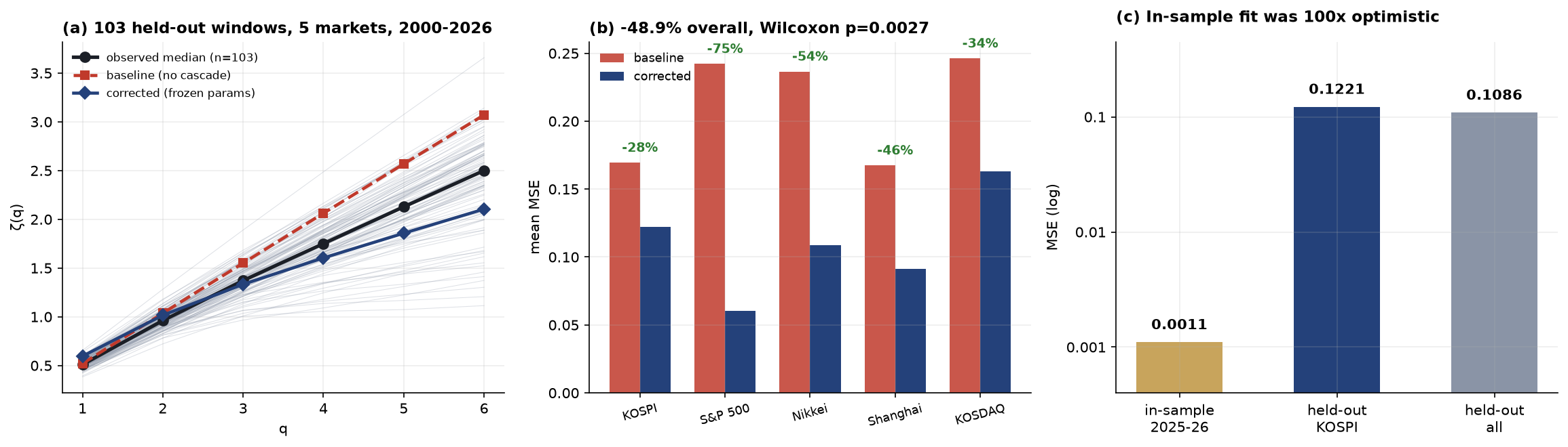
Tuning damping alongside \(K\) drives in-sample error to \(\mathrm{MSE}=0.0011\) on six points with two or three free parameters. Freezing those parameters and evaluating on 103 non-overlapping 310-day windows:
| market | baseline | corrected | improvement | win rate |
|---|---|---|---|---|
| S&P 500 | 0.242 | 0.060 | \(-75.1\%\) | \(81.0\%\) |
| Nikkei | 0.237 | 0.109 | \(-54.1\%\) | \(57.1\%\) |
| Shanghai | 0.167 | 0.091 | \(-45.5\%\) | \(55.0\%\) |
| KOSDAQ | 0.246 | 0.163 | \(-33.9\%\) | \(45.0\%\) |
| KOSPI | 0.169 | 0.122 | \(-28.0\%\) | \(52.4\%\) |
| all (103) | 0.212 | 0.109 | \(\mathbf{-48.9\%}\) | \(58.3\%\) |
Held-out KOSPI error is \(0.1221\) against an in-sample \(0.0011\), a hundredfold gap, and improvement is smallest on the market the parameters came from: median \(\zeta(6)\) across all windows is \(2.500\) against \(2.010\) in the fitting window, so that window is atypical. Refitting on pre-2015 windows and evaluating on 2015–2026 selects \(K=4\), \(R_0=3.0\); the earlier in-sample choice wins only \(46.8\%\) of held-out windows against \(59.6\%\) for the honest refit.
8 From description to forecast, and to portfolio
Reproducing \(\zeta(q)\) constrains an unconditional shape; trading requires a conditional statement, so the two are tested separately. Forecasting realized volatility over \(h\) days with weights estimated only on pre-2015 data:
| \(h\) | single 20-day | EWMA | multi-scale | improvement | markets |
|---|---|---|---|---|---|
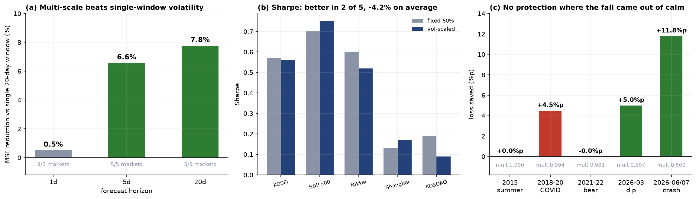
| 1 | 1.4223 | 1.4192 | 1.4150 | \(+0.5\%\) | 3/5 |
| 5 | 0.2525 | 0.2472 | 0.2359 | \(\mathbf{+6.6\%}\) | 5/5 |
| 20 | 0.1529 | 0.1491 | 0.1410 | \(\mathbf{+7.8\%}\) | 5/5 |
Using that forecast to scale a \(60\%\) exposure cap, tightening only, on 2015–2026: mean Sharpe \(0.437\to0.419\) (\(-4.2\%\), better in 2 markets of 5); mean maximum drawdown \(-28.1\%\to-23.2\%\) (\(+4.9\)pp, better in 5 of 5); mean exposure \(0.600\to0.562\). Scaling exposure moves a portfolio along its leverage line, so return and volatility fall together and Sharpe barely moves.
9 Volatility scaling is not tail protection
| episode | drawdown | saved | mean mult. | mult., prior 20d |
|---|---|---|---|---|
| 2015 summer | \(-15.8\%\) | \(0.0\)pp | 1.000 | 1.000 |
| 2018–2020 COVID | \(-43.9\%\) | \(4.5\)pp | 0.994 | 1.000 |
| 2021–2022 bear | \(-34.8\%\) | \(-0.0\)pp | 0.991 | 1.000 |
| 2026-03 dip | \(-19.9\%\) | \(5.0\)pp | 0.507 | 0.658 |
| 2026-06/07 crash | \(-38.6\%\) | \(\mathbf{11.8}\)pp | 0.500 | 0.500 |
Through the COVID decline the book was at full size and de-risked only after the low; through the 2021–22 bear market it never de-risked. Of \(21.3\) percentage points saved, \(16.8\) (\(79\%\)) come from the two 2026 episodes, both of which followed a violently volatile advance and therefore began at the floor. The reason is structural: the forecast reads past realized volatility, so a shock emerging from calm is invisible, and that is the defining property of a tail event.
The mechanism also costs more than the exposure reduction suggests. On the \(20.7\%\) of days when the cap tightened, mean market return was \(+0.229\%\) against \(+0.010\%\) on full-size days: high-volatility regimes contain violent rebounds as well as declines, and a mechanism that cannot distinguish them sits out both.
10 Limitations
The primary window is one unusual episode, with crash and stagnation phases of 27 and 28 trading days, thin for sixth-order moments. Damping ratios depend on an arbitrary \(\omega_0=0.10\), so only inter-phase ratios should be read. Section-3 tests are not corrected for multiple comparisons. The rotation measure is unstable. Circuit results are confined to passive networks; active elements break superposition and were not tested. Higher-dimensional lattices were not tested. Portfolio results isolate the exposure cap with everything else held fixed and do not describe a complete strategy. No result here has been applied to live trading.
11 Conclusion
Tested term by term, the fluid analogy holds in one place and fails in two. It fails as a regime classifier and as a leading indicator. It holds as a statement about scaling, and the term carrying that scaling is identifiable: not device nonlinearity, not topology, not spatial advection alone, but a multiplicative cascade on the driving source. The correction survives out of sample. The portfolio result is the one worth carrying forward: a demonstrably better volatility forecast produced no improvement in risk-adjusted return, and the drawdown improvement it produced was absent in the three largest historical declines. The distance between a better description, a better forecast and a better portfolio is not rhetorical. Each gap was measured here, and two of the three were not crossed.
Data and code availability
All series are public (Yahoo Finance). Every figure and table is reproduced end to end by scripts in https://github.com/waterfirst/ns-capital-flow under analysis/. No proprietary data are used.